SDF Tracking Framework

SDF Tracking Framework

A Python framework for sensor data fusion and target tracking. Built around the formulations in Prof. Wolfgang Koch’s Tracking and Sensor Data Fusion. Every component — motion model, sensor, filter, trajectory, platform — sits behind a small explicit interface and is plug-compatible with the rest.

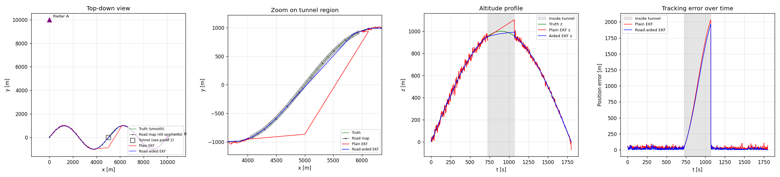
The headline scenario: a 3D mountain pass road with a 2.7 km tunnel midway, two stationary radars at (0, 10 km, 100 m) and (10 km, 0, 100 m), and the target traversing the road at constant speed. Inside the tunnel both radars lose the target; a road-aided EKF keeps the cross-track and altitude estimates close to the manifold while a plain EKF coasts on motion-model prediction alone and drifts. The error spike during the gap is the demonstration; the recovery on re-acquisition is the same filter design, no per-scenario tuning.

219 tests passing · Python 3.10+ · MIT license

Quick start

git clone <repo>
cd sensor-fusion-tracking
pip install -e .

# Run the headline example
python examples/road_with_tunnel.py
# → results/mountain_pass_with_tunnel.png

# Run the full test suite
pytest -v

To launch the interactive scenario builder dashboard:

pip install dash plotly playwright    # not part of the core deps
python -m dashboard                   # serves on http://127.0.0.1:8050

What it does

This framework implements the canonical building blocks of sensor data fusion, in a way meant to be read as much as run. If you’ve taken a tracking course, the names and roles will be familiar; if you haven’t, the inline documentation tries to bridge to the textbook.

The novel pieces are:

• TerrainOcclusion / TunnelOcclusion — a road-aligned tubular occlusion model. Anchored to a PolygonalRoadMap by arc-length range, so the same tunnel definition works on straight and curved roads in 2D or 3D. Composes with DopplerBlindnessOcclusion via CompositeOcclusion.
• PolygonalRoadMap with explicit per-segment arc length (separate from the chord length), so the discretization-error variance σ_d is computed correctly when the polygon under-samples a curved road.
• RoadAidedExtendedKalmanFilter — EKF with a fictitious cross-track measurement from the road map applied at every step, regardless of whether the sensors fired. The mechanism by which the filter coasts through tunnels.
• An interactive Dash dashboard (under dashboard/) that lets you configure the trajectory, sensors, occlusion, filter, and road map through forms, run the simulation, and play back the result in 3D with a time slider — plus export the playback as an MP4.

Components

Motion models (src/sdf/motion_models/)

Sensors (src/sdf/sensors/)

• CartesianPositionSensor — linear; direct noisy position
• RadarSensor — range / bearing / (elevation), with proper angle-wrap on innovation
• GMTIRadarSensor — radar + range-rate, supports a moving Platform

Each sensor optionally carries an OcclusionModel:

• TunnelOcclusion — target in a road-aligned tube → no measurement
• DopplerBlindnessOcclusion — radial-velocity-dependent P_D suppression for GMTI clutter notches
• CompositeOcclusion — OR-composition of several models

Filters (src/sdf/filters/)

• KalmanFilter — linear measurements only
• ExtendedKalmanFilter — local linearization for radar / GMTI
• RoadAidedExtendedKalmanFilter — EKF augmented by a road-map cross-track measurement, applied per step independently of sensor returns
• IMMFilter — Interacting Multiple Models with arbitrary sub-filter list

Scenarios (src/sdf/scenarios/)

• ConstantVelocityTrajectory, MountainPassTrajectory — analytic truth
• PolygonalRoadMap — polygon nodes with surveyed positions, declared σ on node coords, and explicit per-segment arc lengths
• Sensor platforms: StationaryPlatform, StraightFlight, CircleFlight, RacetrackFlight — analytic position and velocity at any t

Visualization (src/sdf/viz/)

• tunnel_wireframe_segments(tunnel) — backend-agnostic line geometry
• draw_tunnel_wireframe(ax, tunnel) — matplotlib helper for 2D or 3D axes

Examples

examples/ contains runnable scripts, each writing a PNG into results/:

Dashboard

The interactive dashboard sits in the top-level dashboard/ directory (deliberately outside the sdf package, to keep Dash and Plotly out of the core dependency tree). It lets you configure a scenario through form fields, run it, and watch the playback.

The scenario builder covers trajectory type and parameters, motion model type and parameters, an add/remove sensor list (each row is its own sensor type with its own form), occlusion model, filter type, road map density and node-position uncertainty, plus simulation seed and time step.

Clicking Run simulation produces:

• A 3D Plotly scene with truth, estimate, sensors, road map, and tunnel, animated frame-by-frame via play/pause and a time slider
• Three side panels: position error vs time, altitude profile, sensor detection timeline
• An Export MP4 button (requires ffmpeg on PATH) that writes the playback to a downloadable video file

Known issues

The dashboard’s scenario builder is more capable than it is correct. Specifically, in its current state:

1. The road map is built and visualized when Enable road map is checked, but the road-aided EKF doesn’t fully consume it through the dashboard path — runs that work cleanly via examples/road_with_tunnel.py show 2 km drift through the dashboard. The example is the reference; the dashboard runner needs an audit.
2. Side panels (error, altitude, detection) don’t sync with the 3D playback’s time slider — they show full time series and don’t move with playback. Fixing this means combining all panels into one Plotly subplots figure so frames are shared.
3. Only ConstantVelocity works as the motion model from the dashboard; other motion models break at runtime due to state-layout mismatches between the trajectory and the filter.
4. Changing the road map’s node-position uncertainty (sigma_nodes) has no observable effect on the tracking error. Most likely a symptom of issue 1.
5. The configured scenario parameters aren’t displayed under the playback; you have to remember what you set.

These are tracked for v7. The core framework (everything under src/sdf/) is verified by the 219-test suite and the example scripts; the dashboard is a viewer on top of that, and its bugs are in the viewer layer.

Layout

src/sdf/                        Core framework (no Dash dependency)
├── core/                       StateLayout, StateDistribution, Measurement, Track
├── motion_models/              CV, CA, CT (known and unknown ω)
├── sensors/                    Cartesian, Radar, GMTI, occlusion models
├── filters/                    KF, EKF, RoadAidedEKF, IMM
├── scenarios/                  Trajectories, road map, platforms
└── viz/                        Visualization helpers (matplotlib + geometry)

examples/                       Runnable demonstration scripts
tests/                          Framework tests (137, all passing)
dashboard/                      Plotly Dash app — outside the package
├── components/                 Spec-based component registries
├── ui/                         Form generator + playback view
├── tests/                      Dashboard tests (82, all passing)
├── schema.py                   ParameterSpec / ComponentSpec / ComponentChoice
├── simulation.py               Config dict → SimulationResult runner
├── mp4_export.py               matplotlib + ffmpeg MP4 rendering
├── app.py                      Dash app + callbacks
└── __main__.py                 python -m dashboard entry point

results/                        Generated PNGs and MP4s (gitignored content)

Architecture principles

Each layer talks to its neighbours through a single interface. A MotionModel only owes the rest of the framework f(x, dt), F(x, dt), and Q(dt), plus a StateLayout describing which indices are which. A Sensor owes h(x), H(x), and a measure() method that handles detection probability and occlusion uniformly. A Filter consumes both through their interfaces and never knows about ground truth.

StateLayout is the small piece of cleverness that holds it together. It decouples state-vector indices from semantics, so a sensor that needs “the position part of the state” can ask the layout for position_idx rather than hardcoding (0, 2) or (0, 2, 4). This is what makes the same Sensor class work for a 2D CV target and a 3D CA target without caring about the difference.

Adding a new filter, sensor, motion model, or trajectory is a single new class implementing its ABC, plus tests; the existing components don’t need to know it exists.

Disclaimer

AI tools such as Gemini and Claude were used in the development of this project.

Attribution

Developed by Fawwaz Bin Tasneem (MSc CS, University of Bonn) as a portfolio project, extending the work done as a part of the course Introduction to Sensor Data Fusion.

Built iteratively across six versions; the architecture (state layout, small interfaces, plug-compatible components) settled around v3 and has stayed stable since. Each release ran a green test suite end to end.

License

MIT.

_{Publishing to GitHub Pages. This repository is structured to serve as its own Pages site: _config.yml at the root configures Jekyll with the minima theme, and README.md is rendered as the index. To enable, go to Settings → Pages, set Source to Deploy from a branch, branch main, folder / (root). No workflow file is needed.}